Counts of brain lesions by MRI in Multiple Sclerosis
Annual relapse rate in pediatric MS
Hospitalizations in heart failure trials
Literature selection:
Keene et al (2007)
Zhu and Lakkis (2014)
Stucke and Kieser (2013)
Friede and Schmidli (2009, 2010)
Schneider, Schmidli, and Friede (2013)
Friede, Häring, and Schmidli (2018)
Mütze, Glimm, Schmidli, Friede (2019a, b)
\(\hspace{1cm}\)
Fixed sample size
\(\hspace{1cm}\)
Blinded sample size reestimation
Group sequential designs
Notation
Let \[
H_0 : \frac{\lambda_1}{\lambda_2} = \delta_0\;,\;\; r = \frac{n_1}{n_2}\;,
\] where \(t_{ijk}\,\lambda_i\) are the rates of a negative binomial distributed random variable \(Y_{ijk}\): \[Y_{ijk} \sim NB(t_{ijk}\,\lambda_i, \phi)\]
This can be derived from the expected Fisher information in a negative binomial regression model (cf., Lawless, 1987, see also Zhu & Lakkis, 2012)
Fixed exposure time
In many applications it can be assumed that all subjects have the same exposure time during the stages of the trial, i.e., \(t_{ijk} = t\). In this case, the information at the end of the trial \({\cal I} = {\cal I}_K\) with \(n_1 = r\,n_2\) simplifies to
Setting \[
{\cal I} = \frac{(\Phi^{-1}(1-\alpha) + \Phi^{-1}(1-\beta))^2}{(\log\frac{\lambda_1}{\lambda_2} - \log(\delta_0))^2} =:
\frac{(z_{1 - \alpha} + z_{1 - \beta})^2}{(\log\frac{\lambda_1}{\lambda_2} - \log(\delta_0))^2}
\] provides the sample size formula \[
n_2 = \frac{(z_{1 - \alpha} + z_{1 - \beta})^2}{(\log\frac{\lambda_1}{\lambda_2} - \log(\delta_0))^2}
\;\left(\frac{1}{t} (\frac{1}{\lambda_2} + \frac{1}{r\,\lambda_1}) + \phi\,(1 + \frac{1}{r})\right)
\] given in Friede and Schmidli (2010) which is the same as approach 2 of Zhu and Lakkis (2014).
\(\alpha\) is replaced by \(\alpha/2\) in the two-sided case (only \(\delta_0 = 1\)).
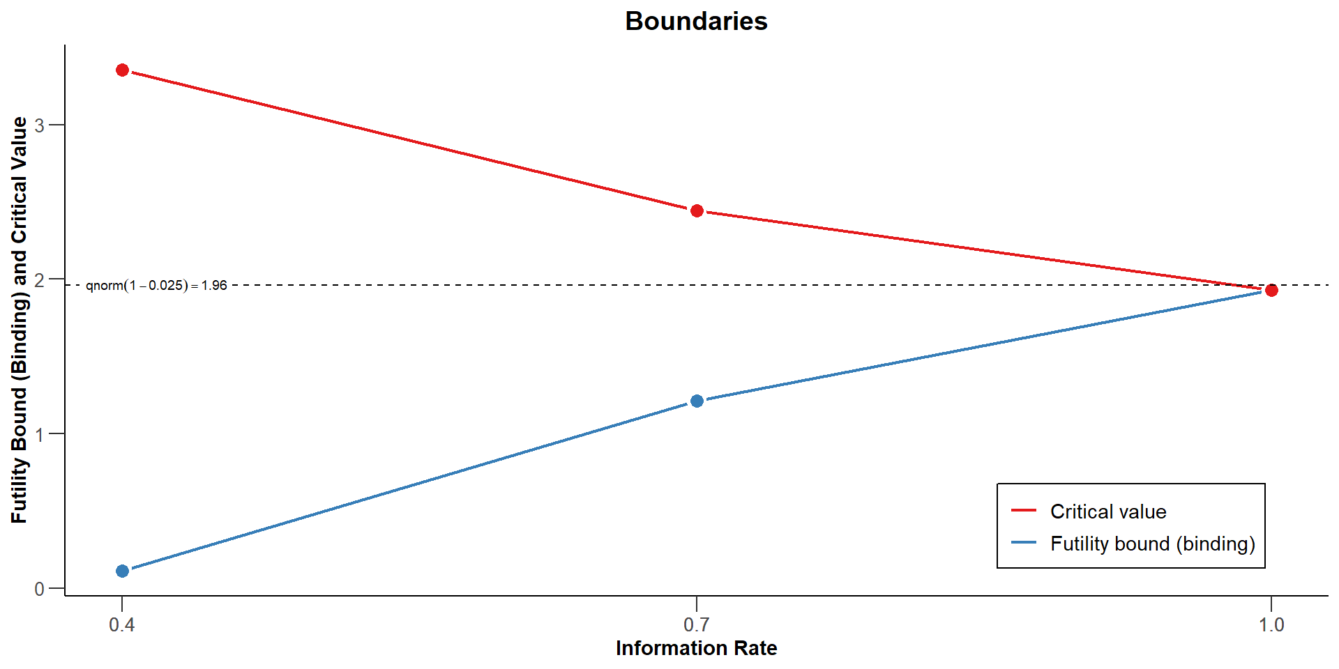
Group sequential design
Test statistic is based on the Wald statistic that adds the difference of the rates on the log-scale.
As shown in Mütze et al. (2019), if Maximum Likelihood estimates are used to estimate the true parameters, the sequence of Wald statistics has the independent and normally distributed increments property (asymptotically).
Maximum sample size
Aim is to calculate the maximum sample size, \(N\), in a group sequential setting.
Fixed exposure time
If a group sequential design with information rates \(I = (\tau_1,\tau_2,\ldots,1)\) and inflation factor \(IF > 1\) calculated, the maximum cumulative sample size is
\[
N = IF\!\cdot\!n_2(1 + r)
\] and \[
N_1 = \frac{r}{1 + r}\!\cdot\! N \;\text{, } \;N_2 = \frac{1}{1 + r}\!\cdot\! N \;.
\]
Variable exposure time
If subjects entering the study have different exposure times, typically an accrual time is followed by an additional follow-up time. If subjects entering the study in an accrual period \([0;\, a]\) and the study time is \(t_{max}\), at time point \(t_k\), the time under exposure for subject \(j\) in treatment \(i\) at stage \(k\) of the trial is
\[
t_{ijk} = t_{k} - a_{ij}\;
\]
with \(t_K = t_{max}\).
The maximum and stage-wise sample size for the group sequential design are found by finding the smallest \(N_{2k}\) (and \(N_{1k}\)) for which
If an accrual time is specified, the calendar times where the interim stages are to be conducted in order to reach the information levels specified for the stages are numerically determined by finding the time points \(t_k\) with
For fixed exposure time and given \(\lambda_1\) and \(\lambda_2\), the optimum sample size allocation ratio \(r\) (minimizing the overall sample size at given power) is given by
\[
r = \sqrt{\frac{\frac{1}{t\,\lambda_1} + \phi}{\frac{1}{t\,\lambda_2} + \phi}}
\] which is found by minimizing
\[
n_2(1 + r) = c \;\left(\frac{1}{t} \frac{(r\,\lambda_1 + \lambda_2)(1 + r)}{r\,\lambda_1\lambda_2} + \phi\,\frac{(1 + r)^2}{r}\right)
\] where \(c\) is a constant.
\(\hspace{1cm}\)
For variable exposure time, the optimum allocation ratio is found by a numerical search algorithm.
Power calculation
At given \(\lambda_1\) and \(\lambda_2\), the non-centrality parameter is
For assuming variable exposure times, at given maximum number of subjects, \(N\),
\[
V = N \left(\frac{1}{
\sum_{j = 1}^{N_1} \frac{t_{1jk}\lambda_1}{1 + \sigma\,t_{1jk}\lambda_1}}
+ \frac{1}{
\sum_{j = 1}^{N_2}\frac{t_{2jk}\lambda_2}{1 + \sigma\,t_{2jk}\lambda_2}}\right).
\]
Power calculation
Given \(N\), the group sequential multiple integral is calculated by setting \[
\zeta_k = \xi \sqrt{t_k\!\cdot\!N} \;,\;k=1,\ldots,K.
\]
R packages for count data:
gscounts: Design and analysis of group sequential designs for negative binomial outcomes, as described by T Mütze, E Glimm, H Schmidli, T Friede (2018)
Each subject is observed the same length of time, or endpoint is event rate in a time interval.
Assume a new combination therapy is assumed to decrease the exacerbation rate from 1.4 to 1.05 (25% decrease) within an observation period of 1 year, i.e., each subject has a equal follow-up of 1 year.
What is the sample size that yields 90% power for detecting such a difference, if the over dispersion is assumed to be equal to 0.5?
Fixed sample analysis, one-sided significance level 2.5%. The results were calculated for a two-sample test for count data, H0: lambda(1) / lambda(2) = 1, power directed towards smaller values, H1: effect = 0.75, lambda(2) = 1.4, number of subjects = 678, overdispersion = 0.5, fixed exposure time = 1.
Stage
Fixed
Efficacy boundary (z-value scale)
1.960
Power
0.9004
Lambda(1)
1.050
One-sided local significance level
0.0250
Usage in blinded sample size reestimation
Superiority Table 1 from Friede and Schmidli (2010)
Given recruitment times and non-uniform recruitment
In getSampleSizeCounts(), you can specify a vector accrualTime and acrualIntensity or specify maxNumberOfSubjects and find study time.
In gscounts, this is handled through the specification of the study entry times (t_recruit1 and t_recruit2).
Example
How long is the study duration if patient recruitment is performed over 1 year instead of 1.25 years, i.e., if 4/5 * 2080 = 1664 subjects will be recruited?