Promising Zone Design with rpact
rpact Training 2024, UCB
August 29, 2024
Binary Example to be Used with and without SSRE
Example Phase 3 study for a skin condition
Binary endpoint
2 analyses (IA at 50% original information),
SSRE using promising zone approach [original or revised version].
Aim to achieve conditional power 30%-90% with the promising zone approach. (Desired overall power = 90%)
Relevant effect size: 0.25
Assumed control success rate: 0.3
Max sample size: 250
\(\alpha\) = 0.025 one sided
Equal allocation between groups
Time to Event example:
Time to disease progression event
2 active arms, 1 control arm
Equal allocation between groups
Power 90%
\(\alpha\) = 0.025 one sided
2 analyses (1 IA at 50% events) futility analysis at interim and select best dose based on highest HR
Assume median TTE in control arm: 25 months
Median TTE in active: 18 months so target HR 0.72
Accrual: Assume 10 for first 10 months, then 20 for next 10 then 30 per month thereafter for max 36 months (or feel free to use a constant accrual rate)
First of all:
Introduction course of Marc Vandemeulebroecke serves as a solid background for the next two hours
For the constrained promising zone approach, see also our vignette
![]()


Load packages
The Promising Zone Approach
Introduction
Chen, DeMets, Lan (2004) have shown that, if at interim the conditional power calculated for the observed effect exceeds 50%, then the test statistic for the group sequential test needs not to be adjusted and the sample size might be increased
Based on this result (and some refinements) Mehta and Pocock (2011) proposed the promising zone approach
Sample size recalculation methods based on conditional power were proposed from the very beginning of adaptive designs (Bauer & Köhne, 1994)
A “constrained” promising zone design was proposed by Hsiao et al (2019)
This design is essentially using the inverse normal combination test because the sample size recalculation procedure is defined in a different way
We consider this design and show how it can be implemented with
rpact.
A Motivating Example from Hsiao, Liu, and Mehta (Biometrical Journal, 2019)
- Efficacy endpoint PFS
- Assumed hazard ratio = 0.67, \(\alpha = 0.025\) and \(\beta = 0.10\) requires 263 events
- 280 PFS events yields power 91.8 %:
getPowerSurvival(
   alpha = 0.025,
   hazardRatio = 0.67,
   directionUpper = FALSE,
   maxNumberOfEvents = 280,
   maxNumberOfSubjects = 350,
) |> fetch(overallReject)
overallReject
0.9178375 Note: maxNumberOfSubjects has no influence on the power calculation
- If 350 patients are enrolled over 28 months with a median PFS time of 8.5 months in the control group, the final analysis is expected to be after an additional follow-up of about 12 months:
getPowerSurvival(
    alpha = 0.025,
    hazardRatio = c(0.67, 1),
    directionUpper = FALSE,
    maxNumberOfEvents = 280,
    maxNumberOfSubjects = 350,
    median2 = 8.5,
    accrualTime = 28
) |> summary()
Power calculation for a survival endpoint
Fixed sample analysis, one-sided significance level 2.5%. The results were calculated for a two-sample logrank test, H0: hazard ratio = 1, power directed towards smaller values, H1: hazard ratio as specified, control median(2) = 8.5, number of subjects = 350, number of events = 280, accrual time = 28, accrual intensity = 12.5.
| Stage | Fixed |
|---|---|
| Efficacy boundary (z-value scale) | 1.960 |
| Power, HR = 0.67 | 0.9178 |
| Power, HR = 1 | 0.0250 |
| Number of subjects, HR = 0.67 | 350.0 |
| Number of subjects, HR = 1 | 350.0 |
| Number of events, HR = 0.67 | 280.0 |
| Number of events, HR = 1 | 280.0 |
| Analysis time, HR = 0.67 | 40.52 |
| Analysis time, HR = 1 | 36.29 |
| Expected study duration under H1, HR = 0.67 | 40.52 |
| Expected study duration under H1, HR = 1 | 36.29 |
| One-sided local significance level | 0.0250 |
| Efficacy boundary (t) | 0.791 |
Legend:
- HR: hazard ratio
- (t): treatment effect scale
- 508 PFS events are needed to have 90% power at HR = 0.75:
maxNumberOfEvents
         507.8443
Clearly, more patients are needed, and a different expected follow-up is calculated.
“Milestone-based” investment:
Two-stage approach with interim after 140 events
Enough power for detecting HR = 0.67
If conditional power CP for detecting HR = 0.75 falls in a “promising zone”, an additional investment would be made that allows the trial to remain open until 420 PFS events were obtained
Otherwise, no additional investment is made, stick to the originally planned event number (= 280)
Conditional power based on assumed minimum clinical relevant effect HR = 0.75.
Constrained Promising Zone Design
Number of additional events for the second stage between 140 and 280
If conditional power for 280 additional events at HR = 0.75 is smaller than \(cp_{min}\), set number of additional events = 140 (non-promising case)
If conditional power for 140 additional events at HR = 0.75 exceeds \(cp_{max}\), set number of additional events = 140, otherwise calculate event number according to \[CP_{HR = 0.75} = cp_{max}\] (promising case)
This defines a promising zone for HR within the sample size may be modified.
E.g.,
- \(cp_{min} = 0.80\)
- \(cp_{max} = 0.90\)
Constrained Promising Zone Design

How do I obtain these plots?
Constrained Promising Zone Design Using rpact
First, define the design
Check simulation
getSimulationSurvival(
   design = myDesign,
   hazardRatio = 0.67,
   directionUpper = FALSE,
   plannedEvents = c(140, 280),
   maxNumberOfSubjects = 350,
   median2 = 8.5,
   accrualTime = 28,
   maxNumberOfIterations = maxNumberOfIterations
) |> summary()
Simulation of a survival endpoint
Sequential analysis with a maximum of 2 looks (inverse normal combination test design), one-sided overall significance level 2.5%. The results were simulated for a two-sample logrank test, H0: hazard ratio = 1, power directed towards smaller values, H1: hazard ratio = 0.67, control median(2) = 8.5, planned cumulative events = c(140, 280), maximum number of subjects = 350, accrual time = 28, accrual intensity = 12.5, simulation runs = 1000, seed = 1886803773.
| Stage | 1 | 2 |
|---|---|---|
| Fixed weight | 0.707 | 0.707 |
| Efficacy boundary (z-value scale) | Inf | 1.960 |
| Stage levels (one-sided) | 0 | 0.0250 |
| Cumulative power | 0 | 0.9290 |
| Number of subjects | 285.6 | 350.0 |
| Expected number of subjects under H1 | 350.0 | |
| Expected number of events under H1 | 280.0 | |
| Expected number of events | 280.0 | |
| Cumulative number of events | 140.0 | 280.0 |
| Expected number of events under H1 | 280.0 | |
| Analysis time | 22.89 | 40.47 |
| Expected study duration under H1 | 40.47 | |
| Conditional power (achieved) | 0.8180 | |
| Exit probability for efficacy | 0 | 0.9290 |
Define the event number calculation function myEventSizeCalculationFunction()
# Define promising zone event size function
myEventSizeCalculationFunction <- function(...,
   stage,
   plannedEvents,
   conditionalPower,
   minNumberOfEventsPerStage,
   maxNumberOfEventsPerStage,
   conditionalCriticalValue,
   estimatedTheta
) {
    calculateStageEvents <- function(cp) {
        4 * max(0, conditionalCriticalValue + qnorm(cp))^2 /
            log(max(1 + 1e-12, estimatedTheta))^2
    }
    #  Note: estimatedTheta is 1 / hazardRatio if directionUpper = FALSE

    # Calculate events required to reach maximum desired conditional power
    # cp_max (provided as argument conditionalPower)
    stageEventsCPmax <- ceiling(calculateStageEvents(cp = conditionalPower))

    # Calculate events required to reach minimum desired conditional power
    # cp_min, manually to be set = 0.80
    stageEventsCPmin <- ceiling(calculateStageEvents(cp = 0.80))

    # Define stageEvents
    stageEvents <- min(max(minNumberOfEventsPerStage[stage],
                           stageEventsCPmax),
                       maxNumberOfEventsPerStage[stage])

    # Set stageEvents to minimal sample size in case minimum conditional
    # power cannot be reached with available sample size
    if (stageEventsCPmin > maxNumberOfEventsPerStage[stage]) {
        stageEvents <- minNumberOfEventsPerStage[stage]

    }
    # return overall events for second stage
    return(plannedEvents[1] + stageEvents)
}
Run the Simulation
by specifying calcEventsFunction = myEventSizeCalculationFunction and a range of assumed true hazard ratios
hazardRatioSeq <- seq(0.65, 0.85, by = 0.01)
simSurvPromZone <- getSimulationSurvival(
    design = myDesign,
    hazardRatio = hazardRatioSeq,
    directionUpper = FALSE,
    plannedEvents = c(140, 280),
    median2 = 8.5,
    minNumberOfEventsPerStage = c(NA, 140),
    maxNumberOfEventsPerStage = c(NA, 280),
    thetaH1 = 0.75,
    conditionalPower = 0.9,
    accrualTime = 36,
    calcEventsFunction = myEventSizeCalculationFunction,
    maxNumberOfIterations = maxNumberOfIterations,
    maxNumberOfSubjects = 450
)
“Usual” Conditional Power Approach
Specify calcEventsFunction = NULL
simSurvCondPower <- getSimulationSurvival(
    design = myDesign,
    hazardRatio = hazardRatioSeq,
    directionUpper = FALSE,
    plannedEvents = c(140, 280),
    median2 = 8.5,
    minNumberOfEventsPerStage = c(NA, 140),
    maxNumberOfEventsPerStage = c(NA, 280),
    thetaH1 = 0.75,
    conditionalPower = 0.9,
    accrualTime = 36,
    calcEventsFunction = NULL,
    maxNumberOfIterations = maxNumberOfIterations,
    maxNumberOfSubjects = 500
)
Comparison of Approaches
aggSimCondPower <- getData(simSurvCondPower)
sumCP <- summarize(
    aggSimCondPower,
    .by = c(iterationNumber, hazardRatio),
    design = "Event re-calculation for cp = 90%",
    totalEvents = sum(eventsPerStage),
    Z1 = testStatistic[1],
    conditionalPower = conditionalPowerAchieved[2]
)
aggSimPromZone <- getData(simSurvPromZone)
sumCPZ <- summarize(
    aggSimPromZone,
    .by = c(iterationNumber, hazardRatio),
    design = "Constrained Promising Zone (CPZ) with cpmin = 80%",
    totalEvents = sum(eventsPerStage),
    Z1 = testStatistic[1],
    conditionalPower = conditionalPowerAchieved[2]
)
sumBoth <- rbind(
  sumCP,
  sumCPZ
) %>% filter(Z1 > -1, Z1 < 4)
What am I Doing Here (20 Simulations)?
What am I Doing Here (20 Simulations)?
aggSimCondPower (excerpt)
iterationNumber stageNumber hazardRatio testStatistic numberOfSubjects eventsPerStage conditionalPowerAchieved
1 1 1 0.65 3.055749872 299 140 NA
2 1 2 0.65 2.147946985 462 140 0.97647736
3 2 1 0.65 2.791088080 286 140 NA
4 2 2 0.65 4.604784960 484 140 0.95739550
5 3 1 0.65 2.273360339 308 140 NA
6 3 2 0.65 2.354898141 500 154 0.90000000
7 4 1 0.65 0.339945318 301 140 NA
8 4 2 0.65 3.394222098 500 280 0.49005084
9 5 1 0.65 3.214083674 292 140 NA
10 5 2 0.65 3.867095531 475 140 0.98399261
11 6 1 0.65 1.927766223 310 140 NA
12 6 2 0.65 3.421863309 500 219 0.90000000
13 7 1 0.65 3.852722577 307 140 NA
14 7 2 0.65 4.474589607 465 140 0.99730594
15 8 1 0.65 1.550133199 292 140 NA
16 8 2 0.65 4.449574478 500 280 0.88203999
17 9 1 0.65 1.486578277 311 140 NA
18 9 2 0.65 3.808874199 500 280 0.86900319
19 10 1 0.65 2.703908473 304 140 NA
20 10 2 0.65 3.532846072 477 140 0.94887592
21 11 1 0.65 2.091238294 298 140 NA
22 11 2 0.65 4.722070782 500 186 0.90000000
23 12 1 0.65 2.943605275 296 140 NA
24 12 2 0.65 4.716717792 465 140 0.96951740
25 13 1 0.65 -0.499247196 295 140 NA
26 13 2 0.65 2.432593895 500 280 0.19375716
27 14 1 0.65 2.610837957 289 140 NA
28 14 2 0.65 1.969946441 466 140 0.93833922
29 15 1 0.65 2.371736530 295 140 NA
30 15 2 0.65 5.372958420 470 140 0.90352112
31 16 1 0.65 1.975357793 287 140 NA
32 16 2 0.65 3.401824564 500 209 0.90000000
33 17 1 0.65 3.026869996 293 140 NA
34 17 2 0.65 3.782438202 469 140 0.97482700
35 18 1 0.65 2.796080259 307 140 NA
36 18 2 0.65 3.783345012 470 140 0.95784632
37 19 1 0.65 2.524581930 302 140 NA
38 19 2 0.65 3.172294909 480 140 0.92712721
39 20 1 0.65 1.196936971 299 140 NA
40 20 2 0.65 3.570700190 500 280 0.79730970
41 1 1 0.75 2.470085788 279 140 NA
42 1 2 0.75 2.236430987 431 140 0.91927751
43 2 1 0.75 2.204008347 292 140 NA
44 2 2 0.75 2.367671894 490 165 0.90000000
45 3 1 0.75 2.794543191 282 140 NA
46 3 2 0.75 4.490879678 450 140 0.95770793
47 4 1 0.75 2.395092736 281 140 NA
48 4 2 0.75 2.227229288 459 140 0.90745342
49 5 1 0.75 2.700123248 289 140 NA
50 5 2 0.75 4.312460477 464 140 0.94847732
51 6 1 0.75 2.194758267 289 140 NA
52 6 2 0.75 1.855574258 473 166 0.90000000
53 7 1 0.75 0.216062465 293 140 NA
54 7 2 0.75 1.153246569 500 280 0.44084615
55 8 1 0.75 0.747564676 303 140 NA
56 8 2 0.75 2.117224473 500 280 0.64902071
57 9 1 0.75 0.501316144 286 140 NA
58 9 2 0.75 2.739216708 500 280 0.55425908
59 10 1 0.75 1.213772140 312 140 NA
60 10 2 0.75 1.477944963 500 280 0.80202747
61 11 1 0.75 0.567341869 302 140 NA
62 11 2 0.75 2.938394897 500 280 0.58021953
63 12 1 0.75 0.530193610 290 140 NA
64 12 2 0.75 1.395018013 500 280 0.56564877
65 13 1 0.75 -1.264623177 281 140 NA
66 13 2 0.75 1.448231116 500 280 0.05160256
67 14 1 0.75 0.378436071 293 140 NA
68 14 2 0.75 0.883424560 500 280 0.50540523
69 15 1 0.75 1.857994818 297 140 NA
70 15 2 0.75 2.633081703 500 232 0.90000000
71 16 1 0.75 1.654564506 278 140 NA
72 16 2 0.75 3.205090849 500 279 0.90000000
73 17 1 0.75 0.647792034 296 140 NA
74 17 2 0.75 1.996768361 500 280 0.61137528
75 18 1 0.75 1.703834619 285 140 NA
76 18 2 0.75 1.740330927 500 266 0.90000000
77 19 1 0.75 1.192409648 290 140 NA
78 19 2 0.75 3.279819482 500 280 0.79602963
79 20 1 0.75 1.504144023 271 140 NA
80 20 2 0.75 3.640154342 500 280 0.87270207
81 1 1 0.85 0.174592408 276 140 NA
82 1 2 0.85 0.968212625 500 280 0.42453925
83 2 1 0.85 -0.426483621 289 140 NA
84 2 2 0.85 1.314187066 500 280 0.21436395
85 3 1 0.85 2.621495325 294 140 NA
86 3 2 0.85 2.320747472 446 140 0.93962554
87 4 1 0.85 0.003110406 284 140 NA
88 4 2 0.85 1.375511813 500 280 0.35875959
89 5 1 0.85 1.945365188 290 140 NA
90 5 2 0.85 3.133356546 500 215 0.90000000
91 6 1 0.85 -1.011310210 288 140 NA
92 6 2 0.85 0.789394462 500 280 0.08438033
93 7 1 0.85 2.081112613 289 140 NA
94 7 2 0.85 2.993868715 500 187 0.90000000
95 8 1 0.85 1.191204214 287 140 NA
96 8 2 0.85 2.607254610 500 280 0.79568799
97 9 1 0.85 0.600912682 284 140 NA
98 9 2 0.85 2.301541734 500 280 0.59329373
99 10 1 0.85 0.331164152 282 140 NA
100 10 2 0.85 1.526268947 500 280 0.48654918
101 11 1 0.85 3.065198083 301 140 NA
102 11 2 0.85 3.308201059 437 140 0.97699712
103 12 1 0.85 0.319882727 286 140 NA
104 12 2 0.85 2.584600483 500 280 0.48205205
105 13 1 0.85 1.173937794 279 140 NA
106 13 2 0.85 1.983222291 500 280 0.79075711
107 14 1 0.85 1.098982145 302 140 NA
108 14 2 0.85 1.347918579 500 280 0.76855470
109 15 1 0.85 1.883605591 288 140 NA
110 15 2 0.85 2.736588475 500 228 0.90000000
111 16 1 0.85 -0.340007504 291 140 NA
112 16 2 0.85 0.836723409 500 280 0.24043802
113 17 1 0.85 1.570731736 281 140 NA
114 17 2 0.85 1.005634342 500 280 0.88606137
115 18 1 0.85 2.448170467 283 140 NA
116 18 2 0.85 2.329024192 446 140 0.91594665
117 19 1 0.85 -0.577379568 297 140 NA
118 19 2 0.85 0.228266524 500 280 0.17302816
119 20 1 0.85 -0.332651632 279 140 NA
120 20 2 0.85 1.610059349 500 280 0.24273297sumCP
   iterationNumber hazardRatio                            design totalEvents           Z1 conditionalPower
1                1        0.65 Event re-calculation for cp = 90%         280  3.055749872       0.97647736
2                2        0.65 Event re-calculation for cp = 90%         280  2.791088080       0.95739550
3                3        0.65 Event re-calculation for cp = 90%         294  2.273360339       0.90000000
4                4        0.65 Event re-calculation for cp = 90%         420  0.339945318       0.49005084
5                5        0.65 Event re-calculation for cp = 90%         280  3.214083674       0.98399261
6                6        0.65 Event re-calculation for cp = 90%         359  1.927766223       0.90000000
7                7        0.65 Event re-calculation for cp = 90%         280  3.852722577       0.99730594
8                8        0.65 Event re-calculation for cp = 90%         420  1.550133199       0.88203999
9                9        0.65 Event re-calculation for cp = 90%         420  1.486578277       0.86900319
10              10        0.65 Event re-calculation for cp = 90%         280  2.703908473       0.94887592
11              11        0.65 Event re-calculation for cp = 90%         326  2.091238294       0.90000000
12              12        0.65 Event re-calculation for cp = 90%         280  2.943605275       0.96951740
13              13        0.65 Event re-calculation for cp = 90%         420 -0.499247196       0.19375716
14              14        0.65 Event re-calculation for cp = 90%         280  2.610837957       0.93833922
15              15        0.65 Event re-calculation for cp = 90%         280  2.371736530       0.90352112
16              16        0.65 Event re-calculation for cp = 90%         349  1.975357793       0.90000000
17              17        0.65 Event re-calculation for cp = 90%         280  3.026869996       0.97482700
18              18        0.65 Event re-calculation for cp = 90%         280  2.796080259       0.95784632
19              19        0.65 Event re-calculation for cp = 90%         280  2.524581930       0.92712721
20              20        0.65 Event re-calculation for cp = 90%         420  1.196936971       0.79730970
21               1        0.75 Event re-calculation for cp = 90%         280  2.470085788       0.91927751
22               2        0.75 Event re-calculation for cp = 90%         305  2.204008347       0.90000000
23               3        0.75 Event re-calculation for cp = 90%         280  2.794543191       0.95770793
24               4        0.75 Event re-calculation for cp = 90%         280  2.395092736       0.90745342
25               5        0.75 Event re-calculation for cp = 90%         280  2.700123248       0.94847732
26               6        0.75 Event re-calculation for cp = 90%         306  2.194758267       0.90000000
27               7        0.75 Event re-calculation for cp = 90%         420  0.216062465       0.44084615
28               8        0.75 Event re-calculation for cp = 90%         420  0.747564676       0.64902071
29               9        0.75 Event re-calculation for cp = 90%         420  0.501316144       0.55425908
30              10        0.75 Event re-calculation for cp = 90%         420  1.213772140       0.80202747
31              11        0.75 Event re-calculation for cp = 90%         420  0.567341869       0.58021953
32              12        0.75 Event re-calculation for cp = 90%         420  0.530193610       0.56564877
33              13        0.75 Event re-calculation for cp = 90%         420 -1.264623177       0.05160256
34              14        0.75 Event re-calculation for cp = 90%         420  0.378436071       0.50540523
35              15        0.75 Event re-calculation for cp = 90%         372  1.857994818       0.90000000
36              16        0.75 Event re-calculation for cp = 90%         419  1.654564506       0.90000000
37              17        0.75 Event re-calculation for cp = 90%         420  0.647792034       0.61137528
38              18        0.75 Event re-calculation for cp = 90%         406  1.703834619       0.90000000
39              19        0.75 Event re-calculation for cp = 90%         420  1.192409648       0.79602963
40              20        0.75 Event re-calculation for cp = 90%         420  1.504144023       0.87270207
41               1        0.85 Event re-calculation for cp = 90%         420  0.174592408       0.42453925
42               2        0.85 Event re-calculation for cp = 90%         420 -0.426483621       0.21436395
43               3        0.85 Event re-calculation for cp = 90%         280  2.621495325       0.93962554
44               4        0.85 Event re-calculation for cp = 90%         420  0.003110406       0.35875959
45               5        0.85 Event re-calculation for cp = 90%         355  1.945365188       0.90000000
46               6        0.85 Event re-calculation for cp = 90%         420 -1.011310210       0.08438033
47               7        0.85 Event re-calculation for cp = 90%         327  2.081112613       0.90000000
48               8        0.85 Event re-calculation for cp = 90%         420  1.191204214       0.79568799
49               9        0.85 Event re-calculation for cp = 90%         420  0.600912682       0.59329373
50              10        0.85 Event re-calculation for cp = 90%         420  0.331164152       0.48654918
51              11        0.85 Event re-calculation for cp = 90%         280  3.065198083       0.97699712
52              12        0.85 Event re-calculation for cp = 90%         420  0.319882727       0.48205205
53              13        0.85 Event re-calculation for cp = 90%         420  1.173937794       0.79075711
54              14        0.85 Event re-calculation for cp = 90%         420  1.098982145       0.76855470
55              15        0.85 Event re-calculation for cp = 90%         368  1.883605591       0.90000000
56              16        0.85 Event re-calculation for cp = 90%         420 -0.340007504       0.24043802
57              17        0.85 Event re-calculation for cp = 90%         420  1.570731736       0.88606137
58              18        0.85 Event re-calculation for cp = 90%         280  2.448170467       0.91594665
59              19        0.85 Event re-calculation for cp = 90%         420 -0.577379568       0.17302816
60              20        0.85 Event re-calculation for cp = 90%         420 -0.332651632       0.24273297
Plot it
ggplot(data = sumBoth,
  aes(Z1, totalEvents, col = design,  group = design)) +
  geom_line(aes(linetype = design), lwd = 1.2) +
  theme_classic() +
  geom_line(aes(Z1, 280 + 200*dnorm(Z1, log(0.75*sqrt(140)/2))),
        color = "black") +
  grids(linetype = "dashed") +
  scale_x_continuous(name = "Z-score at interim analysis") +
  scale_y_continuous(name = "Re-calculated number of events",
        limits = c(280, 450)) +
  scale_color_manual(values = c("red", "orange"))
ggplot(data = sumBoth,
  aes(Z1, conditionalPower, col = design, group = design)) +
  geom_line(aes(linetype = design), lwd = 1.2) +
  theme_classic() +
  grids(linetype = "dashed") +
  geom_line(aes(Z1, dnorm(Z1, log(0.75*sqrt(140)/2))),
        color = "black") +
  scale_x_continuous(name = "Z-score at interim analysis") +
  scale_y_continuous(
    breaks = seq(0, 1, by = 0.1),
    name = "Conditional power at re-calculated event size"
  ) +
  scale_color_manual(values = c("red", "orange"))

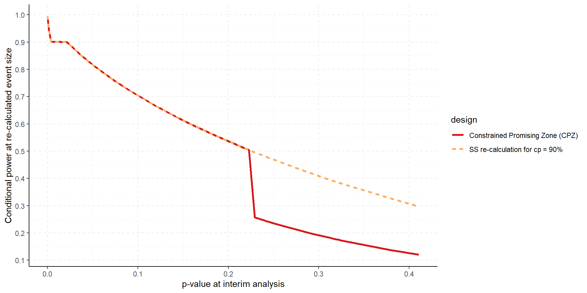
Don’t Increase for, e.g., p = 0.15?

Compare Power and Expected Sample Size
# Pool datasets from simulations (and fixed designs)
simCondPowerData <- with(as.list(simSurvCondPower),
data.frame(
design = "Events re-calculation with cp = 90%",
hazardRatio = hazardRatio,
power = overallReject,
expectedNumberOfEvents = expectedNumberOfEvents
)
)
simPromZoneData <- with(as.list(simSurvPromZone),
data.frame(
design = "Constrained Promising Zone (CPZ)",
hazardRatio = hazardRatio,
power = overallReject,
expectedNumberOfEvents = expectedNumberOfEvents
)
)
simFixed280 <- data.frame(
design = "Fixed events = 280",
hazardRatio = hazardRatioSeq,
power = getPowerSurvival(alpha = 0.025,
directionUpper = FALSE,
maxNumberOfEvents = 280,
median2 = 8.5,
accrualTime = 28,
maxNumberOfSubjects = 500,
hazardRatio = hazardRatioSeq
)$overallReject,
expectedNumberOfEvents = 280
)
simFixed420 <- data.frame(
design = "Fixed events = 420",
hazardRatio = hazardRatioSeq,
power = getPowerSurvival(alpha = 0.025,
directionUpper = FALSE,
maxNumberOfEvents = 420,
median2 = 8.5,
accrualTime = 28,
maxNumberOfSubjects = 500,
hazardRatio = hazardRatioSeq
)$overallReject,
expectedNumberOfEvents = 420
)
simdata <- rbind(simCondPowerData, simPromZoneData, simFixed280, simFixed420)
simdata$design <- factor(
simdata$design,
levels = c(
"Fixed events = 280",
"Fixed events = 420",
"Events re-calculation with cp = 90%",
"Constrained Promising Zone (CPZ)"
)
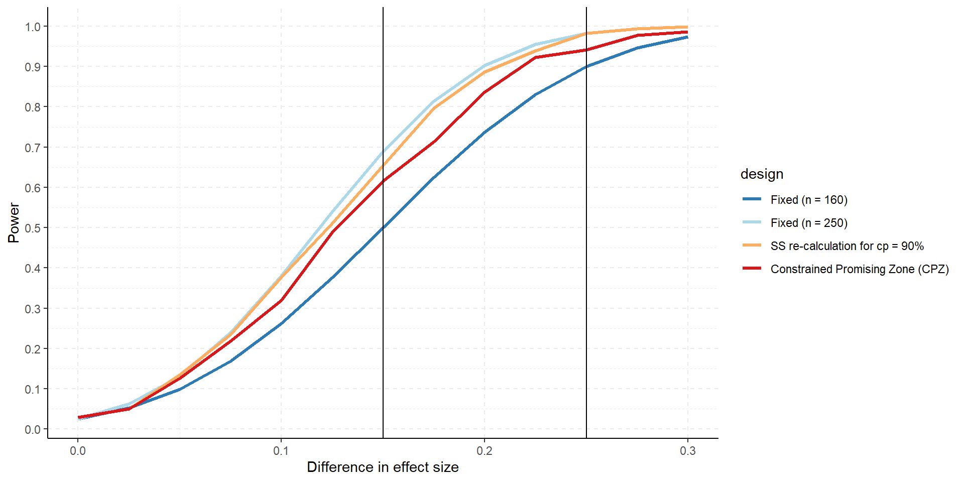
)Difference in Power

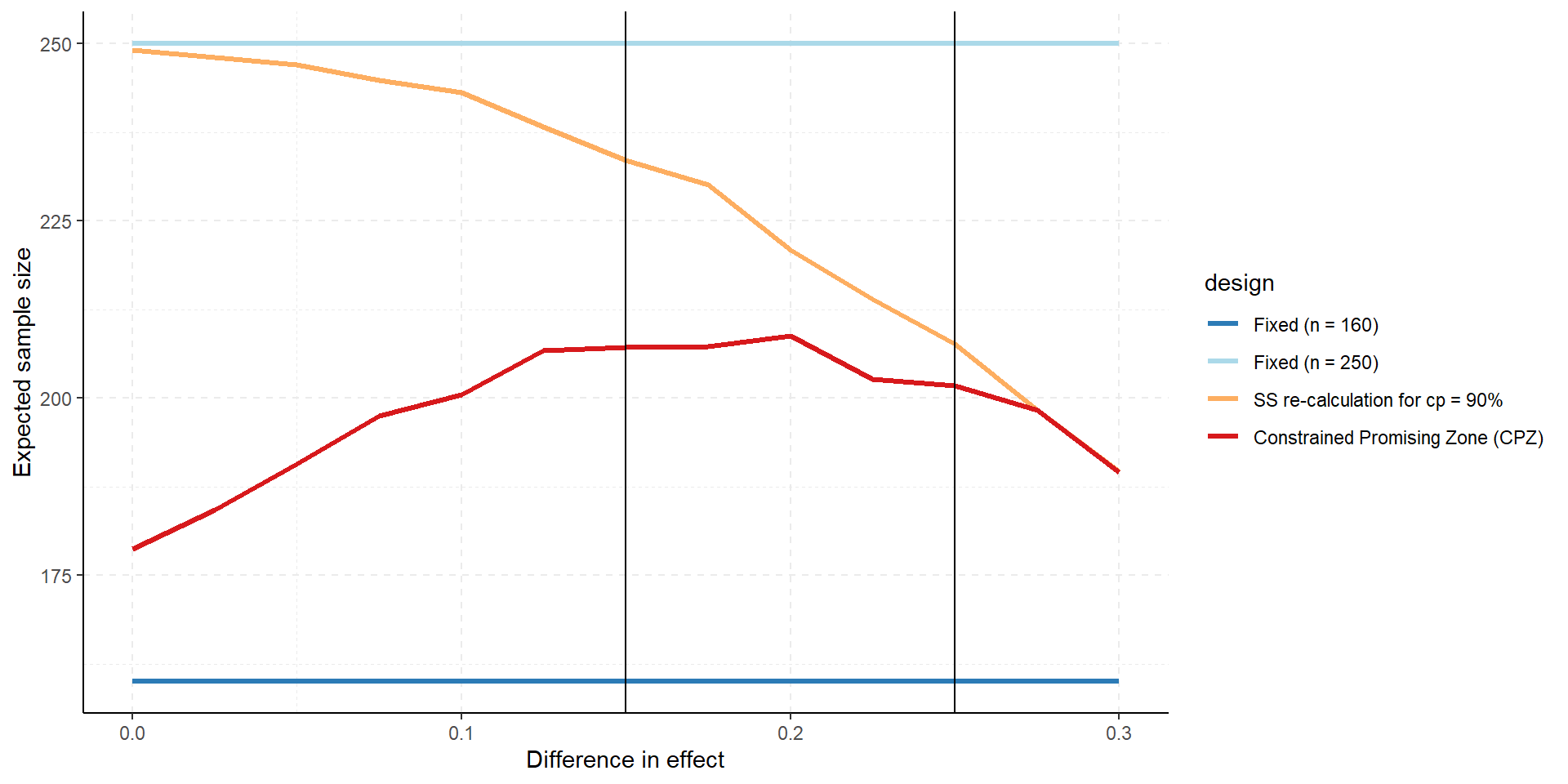
Difference in Expected Sample Size

Summary
- Easy implementation in
rpact - Simulation very fast
- Consideration of efficacy or futility stops straightforward
- Trade-off between overall expected sample size and power
- Change of \(cp_{min}\)?
- Usage of combination test (or equivalent) theoretically mandatory
- Adaptations based on test statistic only.
Application to Binary Case
Example Phase 3 study for a skin condition
Binary endpoint
2 analyses (IA at 50% original information),
SSRE using promising zone approach [original or revised version].
Aim to achieve conditional power 30%-90% with the promising zone approach. (Desired overall power = 90%)
Relevant effect size: 0.25
Assumed control success rate: 0.30
Max sample size: 250
\(\alpha\) = 0.025 one sided
Equal allocation between groups
Sample Size Calculation
Sample size calculation for a binary endpoint
Fixed sample analysis, one-sided significance level 2.5%, power 90%. The results were calculated for a two-sample test for rates (normal approximation), H0: pi(1) - pi(2) = 0, H1: treatment rate pi(1) = 0.55, control rate pi(2) = 0.3.
| Stage | Fixed |
|---|---|
| Efficacy boundary (z-value scale) | 1.960 |
| Number of subjects | 160.1 |
| One-sided local significance level | 0.0250 |
| Efficacy boundary (t) | 0.150 |
Legend:
- (t): treatment effect scale
“Milestone-based” investment:
Two-stage approach with interim after 80 subjects
Enough power for detecting effect 0.25
If conditional power CP for detecting effect = 0.15 falls in a “promising zone”, an additional investment would be made that allows the trial to remain open until 250 subjects were obtained
Conditional power based on assumed minimum clinical relevant effect, 0.15
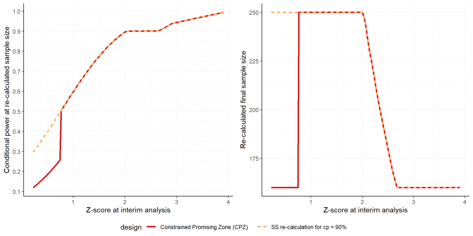
Constrained Promising Zone Design
Number of subjects for the second stage between 80 and 170
If conditional power for 170 additional subjects at effect = 0.15 is smaller than \(cp_{min}\), set number of additional subjects = 80 (non-promising case)
If conditional power for 160 additional events for effect = 0.15 exceeds \(cp_{max}\), set number of additional subjects = 80, otherwise calculate subject number according to \[CP_{effect = 0.15} = cp_{max}\] (promising case)
This defines a promising zone for HR within the sample size may be modified.
Constrained Promising Zone Design Using rpact
First, define the design
Define the sample size calculation function mySampleSizeCalculationFunction()
mySampleSizeCalculationFunction <- function(...,
  stage,
  plannedSubjects,
  conditionalPower,
  minNumberOfSubjectsPerStage,
  maxNumberOfSubjectsPerStage,
  conditionalCriticalValue,
  overallRate
) {
  rateUnderH0 <- (overallRate[1] + overallRate[2]) / 2
  calculateStageSubjects <- function(cp) {
     2 * (max(0, conditionalCriticalValue *
     sqrt(2 * rateUnderH0 * (1 - rateUnderH0)) +
     stats::qnorm(cp) * sqrt(overallRate[1] * (1 - overallRate[1]) +
          overallRate[2] * (1 - overallRate[2]))))^2 /
     (max(1e-12, overallRate[1] - overallRate[2]))^2
  }

  #  Note: change to  max(1e-12, overallRate[2] - overallRate[1]
  #  if directionUpper = FALSE

  # Calculate sample size required to reach maximum desired conditional
  # power cp_max (provided as argument conditionalPower)
  stageSubjectsCPmax <- calculateStageSubjects(cp = conditionalPower)

  # Calculate sample size required to reach minimum desired conditional
  # power cp_min (**manually set for this example to 0.80**)
  stageSubjectsCPmin <- calculateStageSubjects(cp = 0.80)

  # Define stageSubjects
  stageSubjects <- ceiling(min(
    max(minNumberOfSubjectsPerStage[stage], stageSubjectsCPmax
    ),
    maxNumberOfSubjectsPerStage[stage]))

  # Set stageSubjects to minimal sample size in case minimum
  # conditional power cannot be reached with available sample size
  if (stageSubjectsCPmin > maxNumberOfSubjectsPerStage[stage]) {
    stageSubjects <- minNumberOfSubjectsPerStage[stage]
  }
  return(stageSubjects)
}
Simulate Constrained Promising Zone
pi1Seq <- seq(0.45, 0.60, 0.025)
pi2 <- 0.3
n1 <- 80
Nmin <- 160
Nmax <- 250
maxNumberOfIterations <- maxNumberOfIterations

simCPZ <- getSimulationRates(
  myDesign,
  pi1 = pi1Seq,
  pi2 = pi2,
  plannedSubjects = c(n1, Nmin),
  conditionalPower = 0.90,
  # stage-wise minimal overall sample size
  minNumberOfSubjectsPerStage = c(n1, Nmin - n1),
  # stage-wise maximal overall sample size
  maxNumberOfSubjectsPerStage = c(n1, Nmax - n1),
  pi1H1 = 0.45,
  pi2H1 = pi2,
  calcSubjectsFunction = mySampleSizeCalculationFunction,
  maxNumberOfIterations = maxNumberOfIterations,
  seed = 12345
)
Simulate Conditional Power
simCP <- getSimulationRates(
  myDesign,
  pi1 = pi1Seq,
  pi2 = pi2,
  plannedSubjects = c(n1, Nmin),
  conditionalPower = 0.90,
  # stage-wise minimal overall sample size
  minNumberOfSubjectsPerStage = c(n1, Nmin - n1),
  # stage-wise maximal overall sample size
  maxNumberOfSubjectsPerStage = c(n1, Nmax - n1),
  pi1H1 = 0.45,
  pi2H1 = pi2,
  calcSubjectsFunction = NULL,
  maxNumberOfIterations = maxNumberOfIterations,
  seed = 12345
) 
Power and Expected Sample Size Comparison
pi1Seq <- seq(0.3, 0.6, by = 0.025)
pi2 <- 0.3
n1 <- 80
Nmin <- 160
Nmax <- 250
maxNumberOfIterations <- maxNumberOfIterations

simCPLong <- getSimulationRates(
    myDesign,
    pi1 = pi1Seq,
    pi2 = pi2,
    plannedSubjects = c(n1, Nmin),
    conditionalPower = 0.9,
    minNumberOfSubjectsPerStage = c(n1, Nmin - n1),
    maxNumberOfSubjectsPerStage = c(n1, Nmax - n1),
    pi1H1 = 0.45,
    pi2H1 = 0.3,
    maxNumberOfIterations = maxNumberOfIterations,
    seed = 12345
)

simCPZLong <- getSimulationRates(
    myDesign,
    pi1 = pi1Seq,
    pi2 = pi2,
    plannedSubjects = c(n1, Nmin),
    conditionalPower = 0.9,
    minNumberOfSubjectsPerStage = c(n1, Nmin - n1),
    maxNumberOfSubjectsPerStage = c(n1, Nmax - n1),
    pi1H1 = 0.45,
    pi2H1 = pi2,
    calcSubjectsFunction = mySampleSizeCalculationFunction,
    maxNumberOfIterations = maxNumberOfIterations,
    seed = 12345
)


# Pool datasets from simulations (and fixed designs)
simCPData <- with(as.list(simCPLong),
    data.frame(
      design = "SS re-calculation for cp = 90%",
      pi1 = pi1,
      pi2 = pi2,
      effect = effect,
      power = overallReject,
      expectedNumberOfSubjects1 = expectedNumberOfSubjects
    ),
    stringsAsFactors = FALSE
)

simCPZData <- with(as.list(simCPZLong),
   data.frame(
     design = "Constrained Promising Zone (CPZ)",
     pi1 = pi1,
     pi2 = pi2,
     effect = effect,
     power = overallReject,
     expectedNumberOfSubjects1 = expectedNumberOfSubjects
   ),
   stringsAsFactors = FALSE
)

simFixedNmin <- with(as.list(simCPLong),
  data.frame(
    design = paste0("Fixed (n = ", Nmin, ")"),
    pi1 = pi1, pi2 = pi2, effect = effect,
    power = getPowerRates(
      alpha = 0.025,
      sided = 1,
      pi1 = pi1,
      pi2 = pi2,
      maxNumberOfSubjects = Nmin
    )$overallReject,
    expectedNumberOfSubjects1 = Nmin,
    stringsAsFactors = FALSE
  )
)

simFixedNmax <- with(as.list(simCPLong),
  data.frame(
    design = paste0("Fixed (n = ", Nmax, ")"),
    pi1 = pi1, pi2 = pi2, effect = effect,
    power = getPowerRates(
      alpha = 0.025,
      sided = 1,
      pi1 = pi1,
      pi2 = pi2,
      maxNumberOfSubjects = Nmax
    )$overallReject,
    expectedNumberOfSubjects1 = Nmax,
    stringsAsFactors = FALSE
  )
)

simdata <- rbind(simCPData, simCPZData, simFixedNmin, simFixedNmax)
simdata$design <- factor(
   simdata$design,
   levels = c(
     paste0("Fixed (n = ", Nmin, ")"), paste0("Fixed (n = ", Nmax, ")"),
     "SS re-calculation for cp = 90%", "Constrained Promising Zone (CPZ)"
   )
)

Change cp_min (here cp_min = 50%)
Summary
- Easy implementation in
rpact - Simulation very fast
- Consideration of efficacy or futility stops straightforward (e.g., change cp_min)
- Trade-off between overall expected sample size and power
- Usage of combination test (or equivalent) theoretically mandatory.